Why are Chinese models competitive?
Chinese models are low-cost. The likes of DeepSeek, Qwen are trained for up to 40T tokens on models with 30B active parameters (Deepseek claims 37B but that is the amount if they did not use MLA). This takes about $20M of compute at bf16. US companies used to spend more than this on holiday parties (that is, at least until the CFOs found out). So, why aren’t US models better? One reason is that it is hard to effectively use large clusters. Deep learning is quite parallelizable - but not infinitely so. The biggest limit to parallelization is global batch size. You really should take a step every few million tokens. If you have a few thousand GPUs then that means a step every 8k tokens a machine, which is natural. But what happens when you have significantly more GPUs than that?
The first course of action is to increase your batch size. This slows convergence and may even find worse minima for the same number of steps. Think of this like golf. You can play best ball where everyone plays from whichever ball is in the best location. With four people you don’t get a significantly lower score than a single person. If you increase the best ball group to 16 you will see almost no improvement at all over best ball of 4 for 4 times more effort. As seen in the figure below, Anthropic knows this, as Dario wrote a paper and Shuai et. al. from Huawei also reported on this last December.
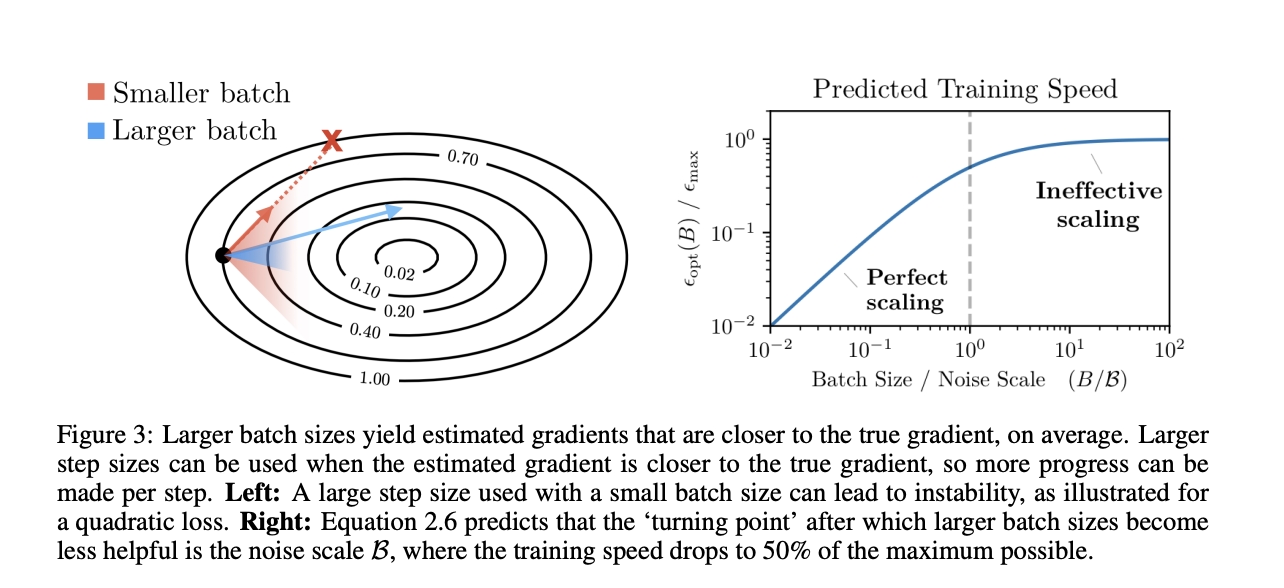
Figure 1: Reproduced from McCandish, Kaplan, Amodei [2018]
So, the US needs another solution. The answer: context parallelism.
Ring Attention, a form of context parallelism, was developed to allow very long contexts that would not fit on a single GPU. A set of GPUs computes attention for a portion of the sequence and they exchange KVs in a ring. Rather than sending 8k (the typical context length) worth of tokens to each machine, we propose using Ring Attention to send far less - as little as 1k, for instance. Then, we can exchange the KVs in order to return to our 8k regular context length. It is through this approach that we can remodel context parallelism for everyday training purposes.
By employing this strategy, we can then scale to 16k GPUs with 2M batch size. This is useful, but where it becomes crucial is when we upsize to 128k GPUs. Now, this allows us to train on that size cluster with a batch size of 4M by using contexts of length 32. Tensor parallelism makes these 256 long, which is just at the limit of what is efficient in GEMMs. Llama 3 405B was trained for 1M steps on 16k GPUs. Reducing the batch size means that we can train the model for 8 times as many steps, whilst using the same data volume.
With a cluster like this, in 90 days we can train a dense 1.6T model. This exceeds the magnitude of the largest openly trained models (Llama 4 Behemoth is 300B active params and Llama 405B a little more) and trained for more than twice as long in terms of tokens and 10 times longer in terms of steps. This would cost about $750M, the price of Lesser Evil Popcorn (the company), three years of Sundar Pichai, or 1/20th of Alexander Wang. Of course, context parallelism comes at a price. But, with a little cleverness, we believe that it can be almost costless.
How? We can either use the IB (the scale out network) which is not that fast so we can only overlap 2x. The natural thing to do is to overlap the all gather of the KV pairs with the computation of Q. Alternatively, we can use a much faster network. DGX boxes come with a NVlink which is 18 times faster, but there is an even faster network-memory. If we use pipeline parallelism we can use context parallelism in time. We process the context forward in the forward pass, storing the KVs in memory, and accessing earlier ones as we move forward. On the backward pass we then carry out the reverse of this process.
This algorithm allows us to add as much context parallelism as the depth of our pipeline permits, but it does limit our pipeline strategies. It requires no networking at all, so is highly efficient.
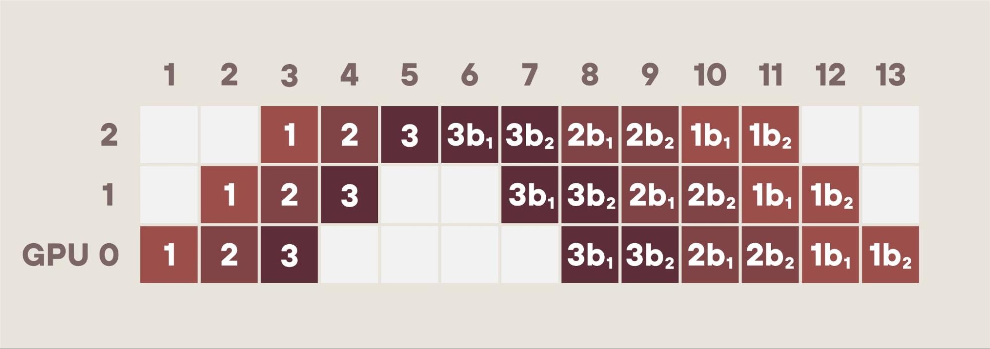
Figure 2: Ceramic’s pipeline adding context parallelism and efficiencies.
Detailed Description of Figure 2: More on Pipeline+Context Parallelism
Boxes labeled 1 are the forward pass of the first 1/3rd of a document.
Boxes labeled 2 are the forward pass of the second 1/3rd of the document.
Boxes labeled 3 are the forward pass of the third 1/3rd of the document.
3b1 Backward pass for last 1/3rd of a document: activation gradients.
3b2 Backward pass computing parameter gradients for the last 1/3rd.
The backward pass is in two parts: 1) gradients of the activations and 2) gradients of the parameters. The forward pass needs previous key value pairs (KVs), the backward pass needs later KV gradients.
In the forward pass for the middle third, box 2 above, we process the middle third of a document and we need the KVs for the first 2/3rds of the document. We compute the KVs for the middle third and we have stored the KVs for the first third in Boxes 1.
For the forward pass, Boxes 2, we need the KVs for the beginning two thirds, but we already stored those KVs while processing Boxes 1.
For the backward pass, Boxes 2b1, we process the gradients for the middle tokens, but need the KV gradients for the last two thirds, but we stored the KV gradients in the last third already while processing 3b1, and we compute the gradients for the middle third.
Training a dense 1.6T model on 128K GPUs.
Returning to training models. For models as large as 1.6T, we use perhaps 160 layers and if we use 4x interleaving this allows us to use a 40 deep pipeline. Our 32 tokens now combine to make a 10k context - using the 8x tensor parallelism of course.
We should check one other issue - our data parallel transfer. Our model is 1.6T parameters. We have a 40x pipeline and 8x tensor parallelism. This makes 320 GPUs hosting each copy of the model so each GPU has 5B parameters.
We use 32 tokens per GPU and 1.6T params so one entire batch will take 6*32*1.6T so 310TFlops. On an H100 this takes 0.6 seconds at a reasonable MFU. If we have 800GB networking this is enough to transfer the model and gradients back and forward as they are 10 G each. With 400GB it would be close but we might be able to manage if we used fp8.
It is hard to go beyond this with DGX boxes and dense models as we have just 256 tokens in our matrix multiplications. We can’t slice any more without losing efficiency precipitously.
We can probably safely scale up a little by using a larger global batch size, but this does not help our data parallel transfer. To solve this NVL 32 or 72s would work and allow us 9x more. However a global batch of 36M is probably several times too large.
Luckily, we don’t have to go down that path, as we use MoEs instead.
In a later blog, I will explain how they face similar but different issues, and can scale up significantly more. There, we can effectively use 1M GPU clusters, even without needing NVL72. This means $6B training runs which approaches the average cost of a government shutdown or the cost of the Phase 5 Marvel movies (Ant Man and the Wasp to Thunderbolts).
Obviously, a good deal.