Revisiting LayerNorm: aka Norms are Important

By Tom Costello, Sean Costello, Lucas Han, and Anna Patterson
The Role of Norms
Normalization techniques are critical in large language model training as they stabilize the learning process by ensuring consistent input distributions across network depths. By standardizing activations, normalizing layers (like Layer Norm) prevent the exploding or vanishing of gradients, thus enabling deeper architectures to converge more reliably and efficiently. This normalization creates smoother optimization landscapes, allowing optimizers like Adam to maintain consistent update magnitudes throughout the network, ultimately accelerating training while improving final model performance.
Beyond training benefits, normalization significantly impacts quantization processes essential for model deployment. Normalized activation distributions are typically better centered around zero with controlled variance, making them more amenable to lower-precision representations with minimal information loss. This characteristic is particularly valuable when converting models from floating-point to integer arithmetic for inference acceleration, as the bounded, well-distributed values experience less quantization error and require fewer bits to maintain performance. This directly translates to models that are smaller in size, faster in execution, and more energy-efficient—critical advantages for practical AI applications running on everyday devices with limited computational resources.
Historically
Layer Normalization was introduced by Ba et al. (2016) as a way of stabilizing hidden state dynamics and speeding convergence. The “Attention Is All You Need Paper”, published one year later in 2017, used Layer Normalization, but in October 2019 both the T5 paper and the RMS norm paper used an RMSNorm. The hugely influential T5 paper did not offer any justification for switching to RMSNorm, but the RMS paper claimed that using the RMS norm was a 64% end to end speedup for certain networks. For the transformers architecture they quoted a 7%-9% speedup, but they were seeing that speedup because they were using the naive tensorflow - 2 pass layer norm. In 2019, this implementation pulled in all of the activations into memory twice – on old GPUs which had small caches - so this was a problem.
T5 used RMS and Google’s PaLM work is descended from T5. LLaMA copied PaLM, everybody copied Llama, so the public models have inherited this decision, but this decision was based on an error. Gemma also inherited from PaLM. Interestingly, GPT2 and 3 say they use LayerNorm. Let’s look at the math.
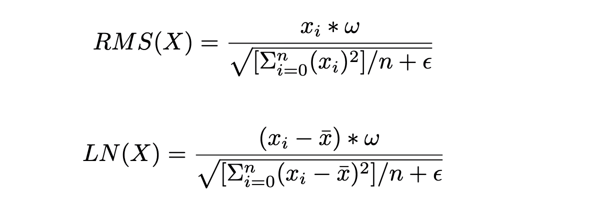
To simplify in practice we can use,

Which is the difference between one and two pass layer norm.
At this point, you might be tempted to use Welford’s algorithm worrying that mean squared will nullify the prior sum. High end CUDA uses Welford, but the square of the mean is always small compared to the variance in practice, so Welford is not appropriate for training as it adds extra divisions that add no benefit in practice. More discussion on precisely why this is not a practical concern when comparing to RMSNorm is included in the appendix.
And so mistakes were made and people just copied the mistakes downward.
In our study, described herein, Layer Norms are always faster or tied in performance and they have the great property of being centered at 0 which helps precision. We examine this in detail in our experiments described herein.
Naive Pytorch:
When the RMSNorm paper was published in 2017, they were comparing a RMSNorm implementation written in Pytorch/Tensorflow with a LayerNorm also written in Pytorch/Tensorflow. With this sort of approach, the differences in performance between RMSNorm and LayerNorm are huge.
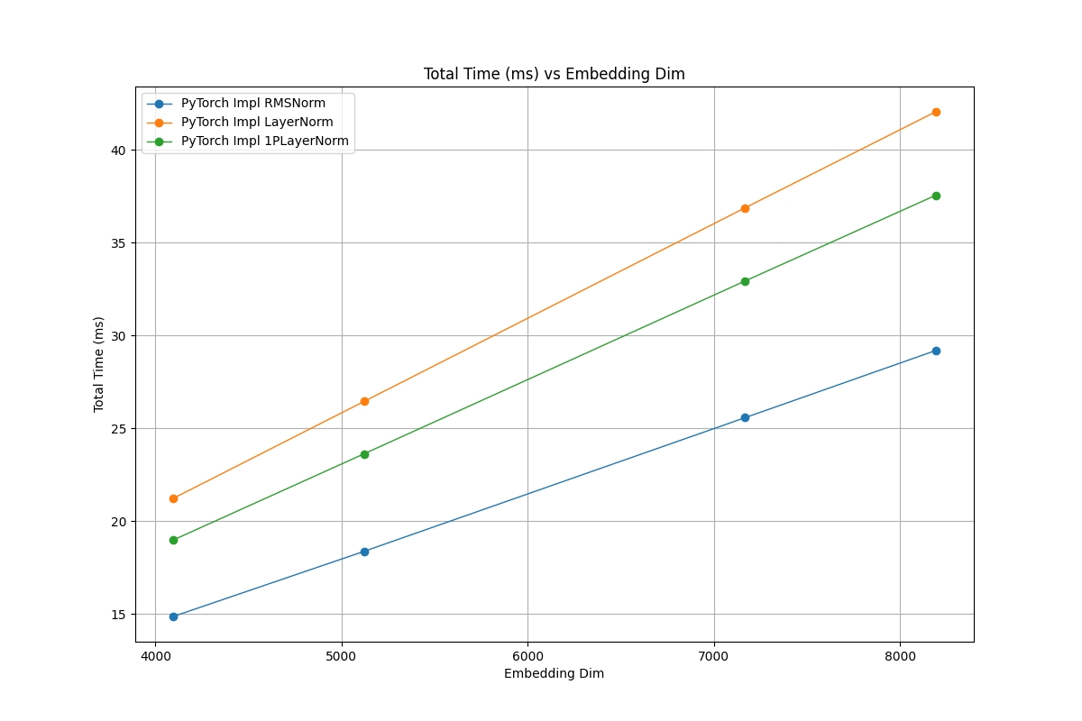
Naive Pytorch Implementations
As you can see in the above figure, the difference in performance between RMSNorm and LayerNorm can be up to 40%. We also included a 1 Pass implementation of LayerNorm that calculates the resulting variance as Var(x) = x2-μ(x)2 which is a simplification but also increases the overall speed as can be seen in the chart above.
When T5 was being written, the performance of the normalization layers was even more important than it is in today’s modern models, as the T5 models were all relatively small by modern standards. The relative performance of normalization scales with the size of the activations (Batch Size, #Tokens, Embedding Dim), whereas the matrix multiplies of the attention and MLP modules scales with Embedding Dim2 Batch Size # Tokens. This means that as the size of the model increases, the relative importance of norm performance decreases.
Activations Aren’t Centered:
One main concern with modern model training is its ability to be quantized to low precision formats. Low precision formats such as fp16 and fp8 have their best precision centered around 0 and lose precision quickly towards the outside of their range. As such it is important that all model parameters and activations be centered around 0. When examining pretrained models that were trained with RMSNorm, we find that the activations do vary from a Mean of 0. The mean difference from 0 varies greatly especially in later layers.
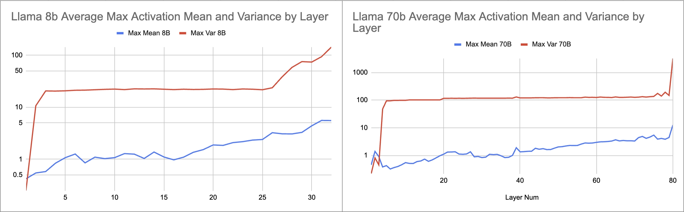
Activation Distributions
We see here in the graph above our observations about the distribution of activations in trained LLama3 models. These numbers are measured as being the average of the maximum token mean (calculated as torch.max(torch.mean(activation,dim=1))) for 4 intermediate values in each layer. These values are the output of both RMSNorms, the output of attention and the output of Swiglu. As you can see, the mean of the activations increases significantly within the first few layers and continues to grow quickly into the deeper layers spiking massively in the last few layers.
This problem is less of an issue in shorter runs as the initialization around 0 or 1 for the weights still holds significant sway. As a result in short runs, RMS and LayerNorm give similar results, because it would take a longer run to see the stabilization of LayerNorm make a difference. However, quantization effects are seen immediately. This issue was less of a concern when RMSNorm was proposed as the initial RMS Norm experiments were done in float32, on old GPUs, but now with bf16 and fp8 centering around 0 is more important.
Modern Methods
Currently, there are 3 potential methods for optimizing performance over a simple Pytorch implementation. The first is to use the Pytorch optimized code for LayerNorm which is contained in torch.nn.LayerNorm. This is quite fast by itself. The second method is to wrap your Naive Pytorch implementations in torch.compile which attempts to compile the implementations in order to speed them up by fusing operations. The last method is to use optimized Triton Kernels in order to specify how the operations should be run on the GPU.
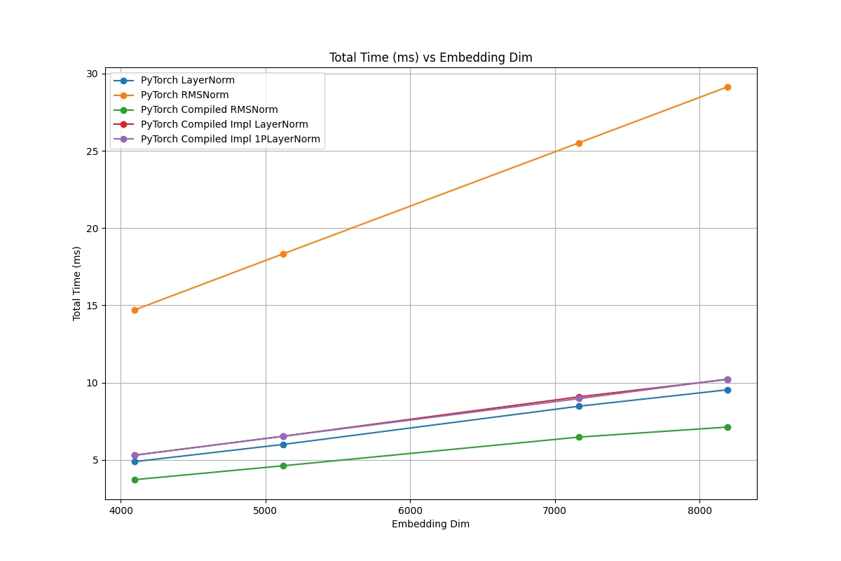
Compiled Pytorch vs Optimized Pytorch vs Naive Pytorch
The above chart shows the performance of torch.nn.LayerNorm vs. torch.nn.RMSNorm, vs. the compiled modules with the implementation. As you can see the slowest implementation by far is PyTorch RMSNorm — this is essentially just the naive implementation with no obvious fusing or compilation. Next slowest is the compiled versions of Pytorch LayerNorm and Pytorch 1Pass LayerNorm — these become almost identical in performance once compiled but are much faster than they were before compilation. The second fastest implementation is the standard PyTorch, torch.nn.LayerNorm — this is backed up by optimized kernels inside of Pytorch and boasts strong performance. The fastest implementation in this graph is the compiled RMSNorm, which goes to show the performance speedups that it can be capable of. However, when triton is taken into consideration a very different picture is drawn.
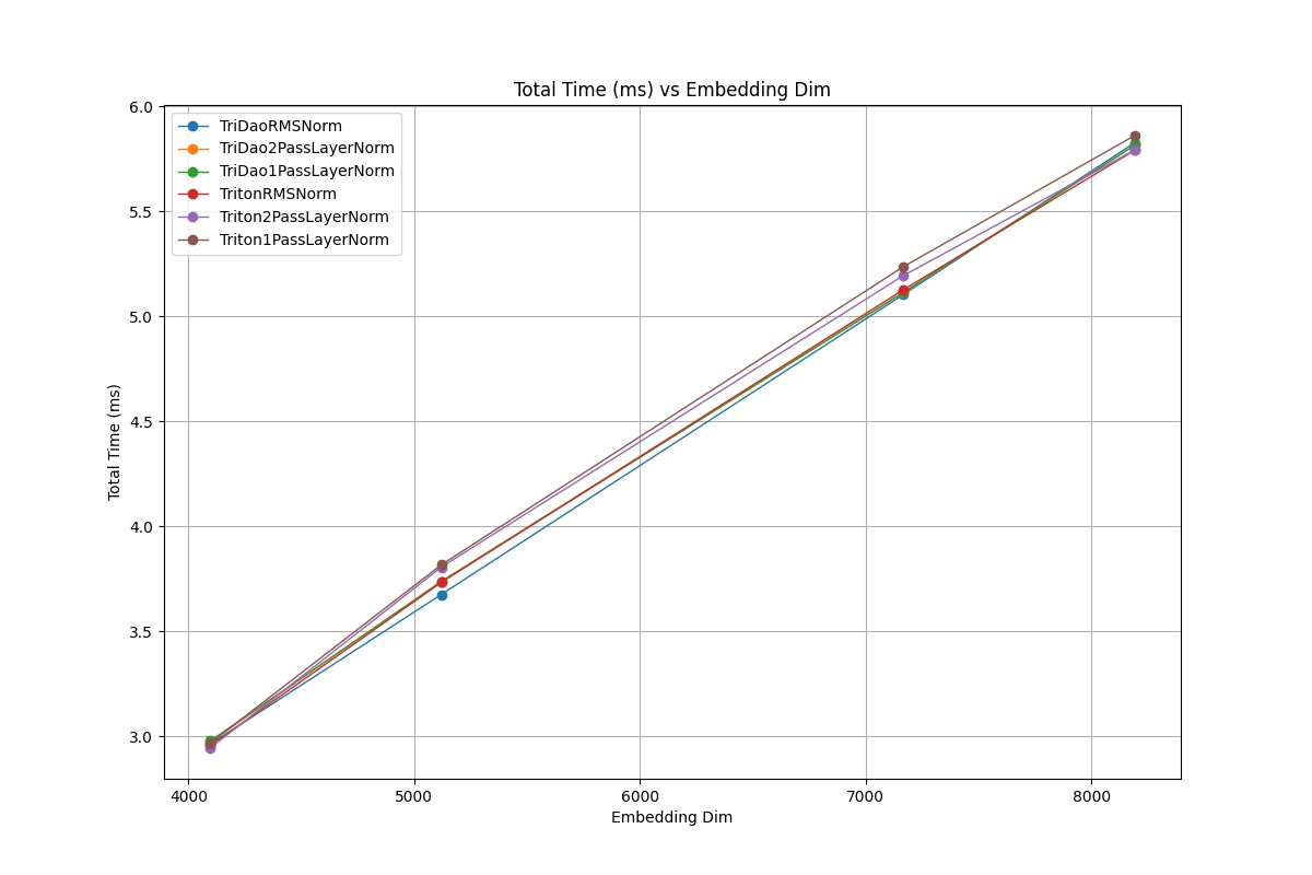
Triton Implementations
Every triton implementation on LayerNorm, RMSNorm or 1Pass LayerNorm has nearly identical performance on every dimension size while outperforming all of the other methods we have tested on every tested dimension size. As such when trying to get the best performance out of our normalization we find that there is no significant difference in performance between LayerNorm and RMSNorm.
Convergence Analysis
LayerNorm vs 1 Pass LayerNorm vs RMSNorm
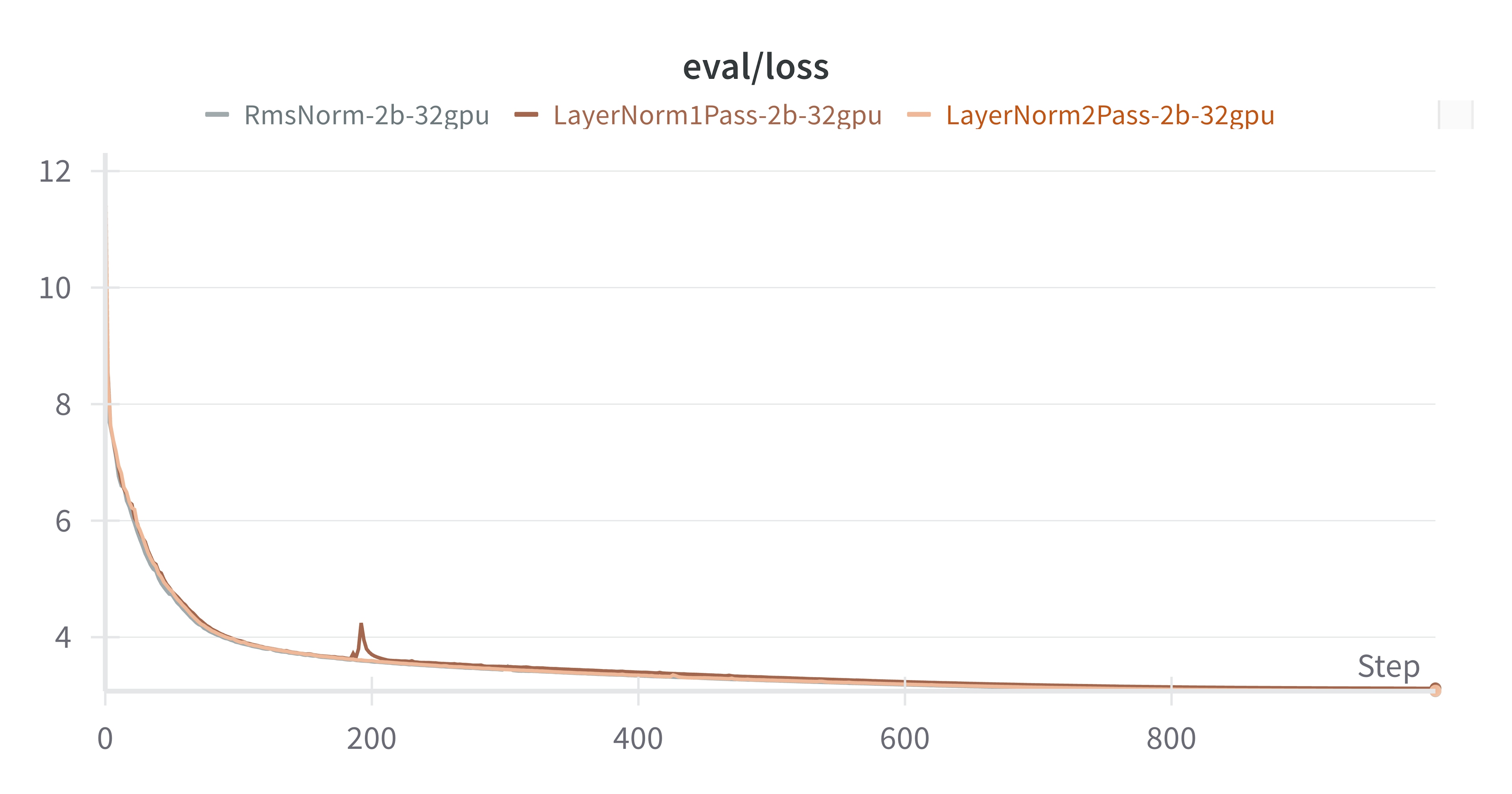
We tracked the evaluation loss (eval/loss) throughout the training process for the three configurations: RmsNorm-2b-32gpu, LayerNorm1Pass-2b-32gpu, and LayerNorm2Pass-2b-32gpu. These were each trained with the triton optimized kernel for their particular algorithm.
The graph clearly shows that the convergence behavior was remarkably similar across all runs, with all runs resulting in an evaluation loss between 3.0 to 3.15.
Conclusion: Historical Accident
Overall, LayerNorm is superior compared to RMSNorm, due to its stability and its compatibility with quantization. While in the past RMSNorm was believed to be superior in performance compared to LayerNorm, we have observed that it is not the case today in practice.
Using the increased cache size, modern toolings and architecture evolutions, the performance gap between RMSNorm and LayerNorm has closed to nothing. As a result, we would recommend that anyone contemplating which norm to use in their architecture should choose LayerNorm.
Appendix
Evaluation
Performance Latency Benchmark
To quantify the practical speed differences between LayerNorm and RMSNorm variants, we conducted latency benchmarks. We measured the forward pass time, backward pass time, and total time (forward + backward) in milliseconds for each implementation. The tests covered configurations relevant to Transformers:
- Sequence Length: 8192
- Embedding Dimensions: 4096, 5120, 7168, 8192
- Batch Size: 4 per GPU
- Hardware: NVIDIA A100 80GB
- Precision: Float32
The implementations include PyTorch built-in modules/methods, naive PyTorch using PyTorch operations, compiled PyTorch, and Triton kernels from various sources.
Benchmark Results
The detailed table of results can be found in the LayerNorm vs. RMSNorm table.
On Welford’s
Welford’s algorithm is the idea of collecting not the running mean and variance but the sum of squares of differences from the current mean. This can be done with a running count of the number of samples so far and some divisions, but this makes it more complicated and slower than simply collecting the sum of the squares and the running mean. Welford’s avoids catastrophic cancellation, which is useful in other applications but as activations are centered around 0, is not an issue in transformers.