What’s actually different about GPT-OSS?
Written by Tom Costello & Yu-Chi Hsu
OpenAI released open models last week, the first open weight model that they have released since GPT3.
This architecture exhibits three major differences from the usual Transformers++ recipe that PaLM, Llama, Qwen, and other models of this variety have used:
1. OSS uses the idea of fine-grained experts, but without DeepSeek’s shared expert.
2. OSS uses sliding attention, but, to tackle the issue where deleting the first token confuses the model, they add an attention sink, a token that is always present and absorbs attention without contributing to the net results.
3. Strikingly, OSS clips both the gate and up matrices in SwiGLU, shifts the output of the up matrix, and scales the outputs of the gate matrix. In their implementation, there are 5 new constants with inline numbers set to obscure values like 1.702 and +7.0.
Whilst the first two changes have been widely discussed, so far popular discourse has neglected to address the changes in SwiGLU.
In general, changes in model architecture are fairly rare, as releases from major labs tend to replicate other labs’, using their architecture as a blueprint. As such, any changes to model configuration are significant. OpenAI’s new work has piqued our interest, and so we think that it deserves a deeper dive.
The Attention layer has been subject to countless propositions of change. However, there has been widespread adoption of SwiGLU as the default MLP layer, so it’s exciting to see developments in the MLP layer space.
But, before we look at actual data, let’s do a little speculation. Why clip the outputs of matrices? Presumably, at later layers, there are a few huge outliers, and clipping keeps them under control. Previous research has found it beneficial to clip all initial parameters to 3 std devs. For example, at initialization Olmo clipped parameters to 3 std dev, and found that this prevents loss spikes after hundreds of billions of tokens. Obviously, the number 7 is larger than 3 but we think the same reasoning applies. Outliers can be harmful, so you want them, but not too much. 7.0 is actually very large when you consider that the input to each matrix is normalized to 1.0. This is comparable to a z-score of 7, which corresponds to men over 7ft 5inches tall. These people exist, but are notable. There are perhaps only 10 NBA players this tall.
As we go to higher layers, the number and size of outliers increase. However, the residuals also increase in outliers. Does this mean we should keep the same clipping threshold at all layers? If the purpose of clipping is to control outliers so they are comparable to the residual, we might expect the clipping to be tighter at lower layers but to relax so that it matches the residual stream.
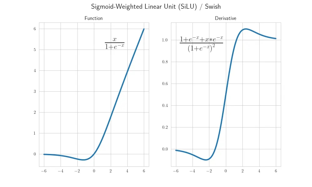
Scaling the input to SiLU makes it sharper, so more alike to GeLU. OpenAI had always favored GeLU while Google has comparatively pushed sigmoid. If one were better than the other, we would expect to know this distinction by now.
The difference is mostly found in the width of the nonlinear bumps. It is fascinating that OpenAI stuck with GeLU rather than SwiGLU, and this demonstrates that there still is a “culture” in labs. Interestingly, the initial proposal for swish suggested a learnable beta, but this was not used in the paper, and has attracted little attention since. Below is a basic Picture of SiLU, and also shifting the output of the up matrix is weird, but perhaps it can be explained by the multiplicative identity being 1.0 rather than 0.0?
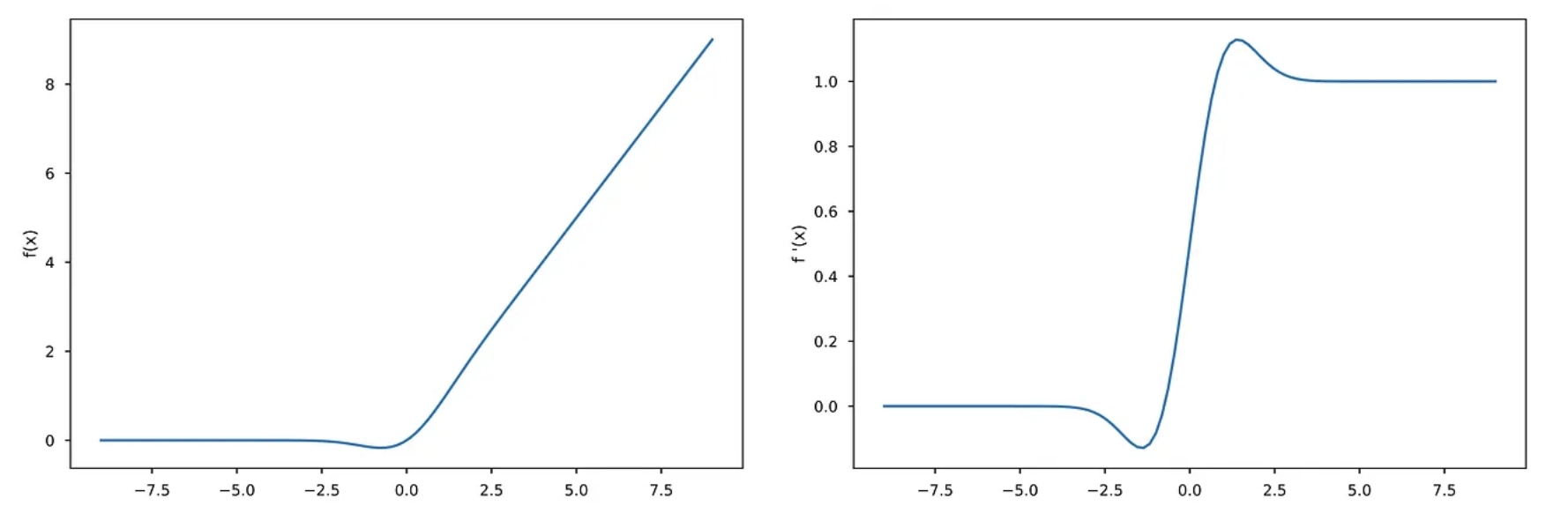
GeLU and GeLU’s derivative.
If the output of the up matrix is evenly distributed around zero, then adding 1.0 moves the average value from 0.0 to 1.0 - so multiplying by it makes no change. If the values are tightly grouped around 0.0 then this allows most of the up values to have no effect. Is this a good idea? Maybe. Personally, I would have expected the values below one to be distributed in the range 0 to 1, where x is as likely as 1/x. Maybe I will get someone to try that experiment out later.
So, we can think of the three changes that OpenAI made as being a somewhat natural progression: they use GeLU rather than sigmoid, they clip to prevent outliers, and they move the up so its default is to be the identity. Each of these changes are reasonable, but they do introduce three places where we are unsure what the best approach is. Luckily, we have a way of finding out which way is right - we can learn what values work best.
Before we experiment, let’s call our shots. We expect clipping to become wider at higher layers to match the residual. We expect GeLU to be more effective at low layers and SiLU to be more effective at higher layers. GELU has a wide bump, so it might be better at noisier signals, while layers with more refined features will want a more compressed bump. We expect the multiplier 1.0 to make most sense at the last few layers. At earlier layers, we care more about creating new signals rather than refining the existing data, so the naturalness of the multiplicative identity might be less important than the greater expressive power of centering around zero.
So, why don’t we train a model and see what values are best? Normally, we make all layers the same, but here our intuition is that different functions will do better at different layers. We can’t train a hard threshold, so we replace them with a sigmoid.
But, before we do this, let’s see if Open AI’s new SwiGLU is better than SwiGLU Classic. As one would expect, Classic wins slightly - never bet against Noam when it comes to choosing hyperparameters. You’ll see this in the final val/loss graph of this blog.
So, onto the experiments.
First, we look at the scaling factor alpha that can change a SiLU into a GeLU. We train a Qwen3 0.6B model over C4 for the recommended Chinchilla 20x the number of parameters, tokens. The Qwen3 model is perhaps the latest dense model and includes QK norm and is deeper and narrower than earlier models, but otherwise retains the standard Transformers++ architecture. We vary alpha, and find a very strange pattern: layer 0 likes alpha to be 1.0, so to act like a traditional SiLU. Layers 1 through 4 like a higher alpha, so act more like a GeLU, but in a smooth linear down ramp from 1.4 to 1.1. After layer 4, the model prefers alpha to be below 1.0 (so further from GeLU than SiLU is) and then it smoothly reduces far below 1.0 to 0.4 at layer 26. The last layer, like the first, is an outlier, and was the layer that stabilized most slowly. It ended up at 0.6, again, below SiLU.
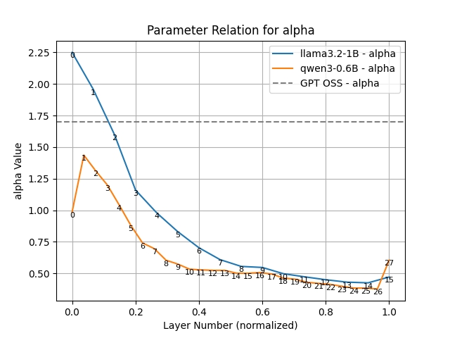
Graph of Alpha Layer
This is shocking, as it suggests that different layers benefit from different-shaped non-linearities.
Normally, a result like this would almost certainly be noise, but the pattern is reproducible across models (Llama models show the same pattern) and the increase in alpha by layer is smooth. This suggests that this is a real phenomenon.
What could explain this? Most likely, this has to do with either the kurtosis of the input (how skewed towards outliers it is) or the shape of the gradients flowing backwards. Earlier, we hypothesized that it would happen due to more and less refined features at earlier and later layers. In hindsight, if an LLM told me that, I would think it was hopelessly vague.
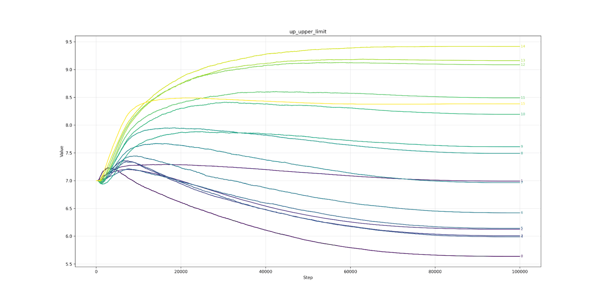
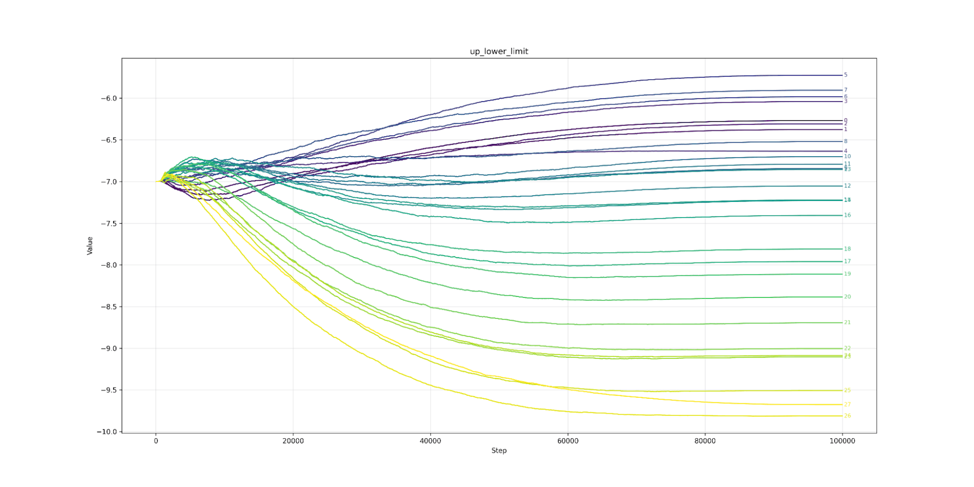
Let’s look at clipping next. Here we find that lower layers prefer tighter clipping. Layer 7 (the strictest) would like to be clipped at 6.0 (or about 7ft 2’ for men) while layer 26 (the loosest) would clip at over 10.0 (8ft 4’ an inch taller than Sultan Kösen the tallest living man). The clipping value from layer 7 to 26 is almost a straight line. The same pattern appears in Llama (from layer 3 onwards). As we predicted, the model likes looser clipping at high layers and tighter at lower. As expected, the lower limit is the mirror image of the upper.
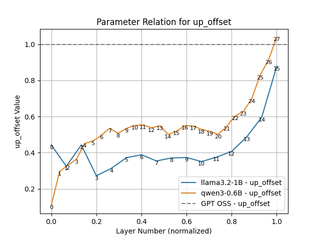
Up Offset
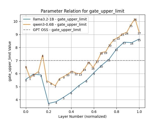
Gate Upper Limit Clipping
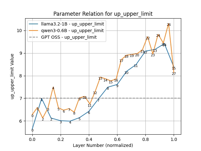
Up Upper Limit Clipping
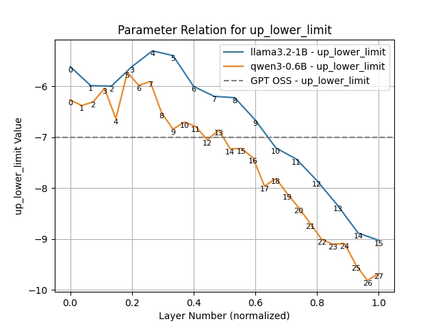
Up Lower Limit Clipping
How about the gate? Like OpenAI, we just clipped at the high end. The low end is clipped by the sigmoid around 0. There we see the same pattern of tighter clipping at low layers and looser at higher. The clipping is even more extreme, going as low as 3.7 for Llama layers (a meagre 6ft 9 - LeBron James?).
That leaves our last parameter: shifting the output of the up-matrix? Again, we see a pattern. Layer zero hates the shift and would like it to be 0.1 (possibly heading towards 0). As we travel up in layers, the preference for the shift increases, until at layer 27 it is slightly over 1. As we predicted, the multiplicative identity makes more sense for higher layers. Strangely, most layers cluster sound 0.55, somewhere in the middle. I can’t explain this phenomenon.
Overall, we see different layers want different slopes inside the sigmoid, different offsets for the up, and different clipping.
These changes actually improve our loss, showing a lower loss. With our experiments and varying these parameters to learned numbers, perhaps we get to the same loss 20% faster. This is definitely a win.
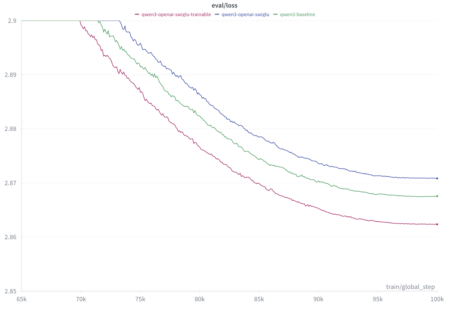
Graph of loss curve of Qwen3
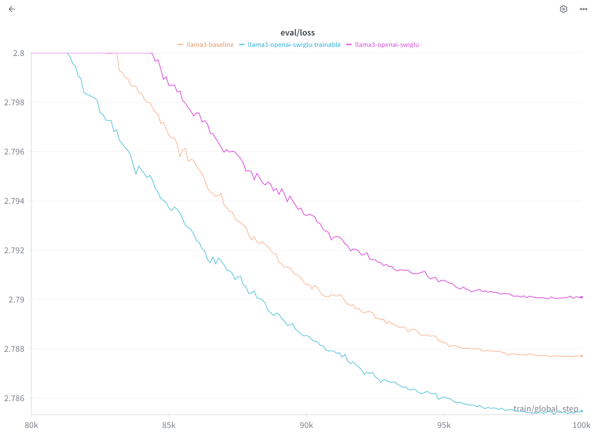
Graph of loss curve of Llama3
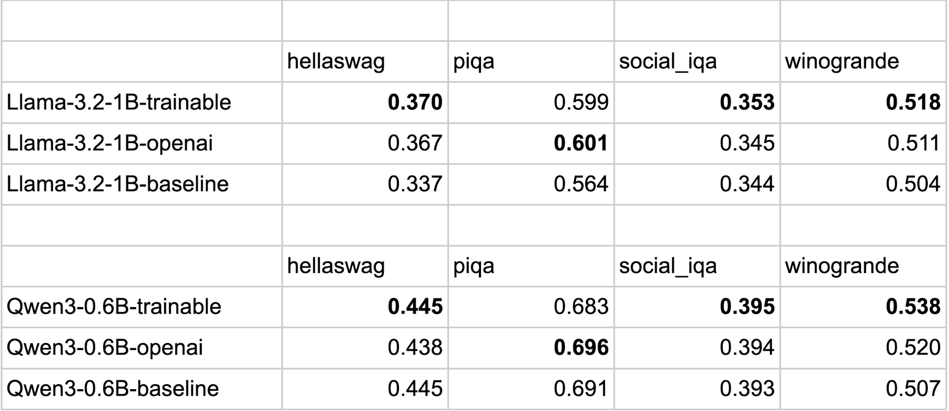
Above are the Eval Results
Finally, there is room to modify the setting in SwiGLU. We did not find a single set of parameters that improves over SwiGLU. That would involve beating Noam’s defaults, which he explains as follows: “We offer no explanation as to why these architectures seem to work; we attribute their success, as all else, to divine benevolence.” However, if we vary some constants per layer, then we can identify a definite win. It seems that, as Benjamin Franklin was fond of saying, “God helps those who help themselves.”
Thanks also: Dr. Anna Patterson and Lucy MR Phillips for their contributions.
Implementations:
OpenAI OSS implementation
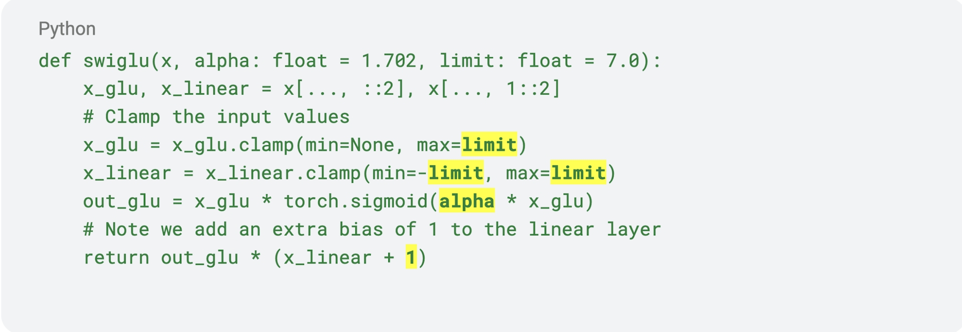
We made these 5 hyper-parameters trainable
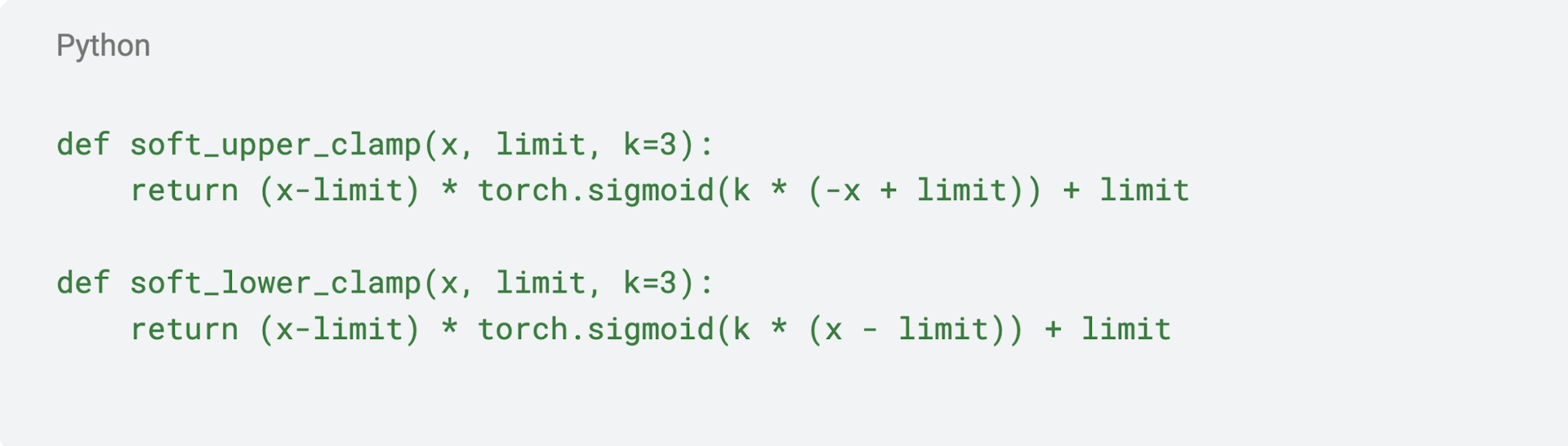
Also we used smooth clamps:
So the actual forward looks like this:
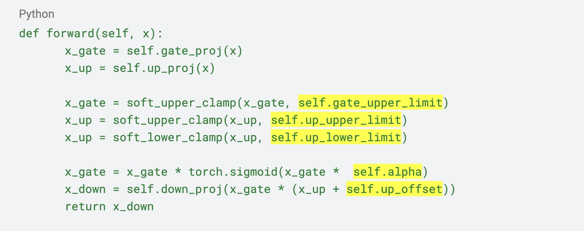
The highlighted variables are trainable are interesting graphs below:
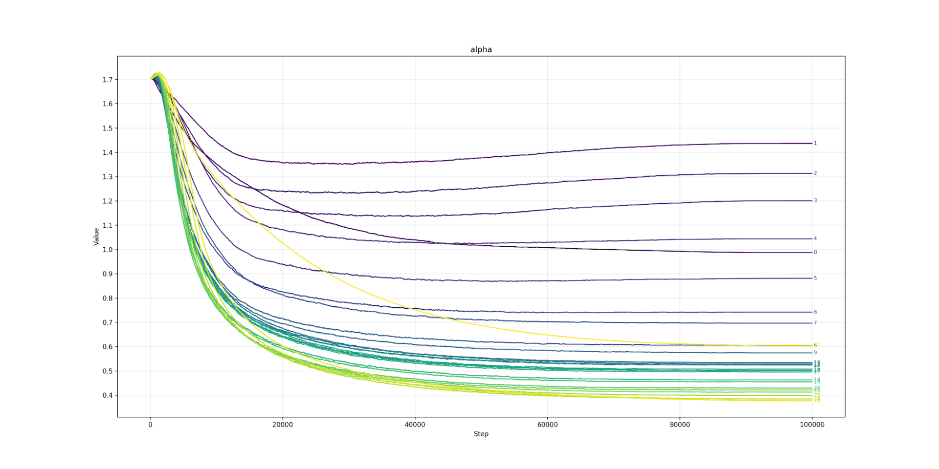
Alpha Qwen3 0.6B
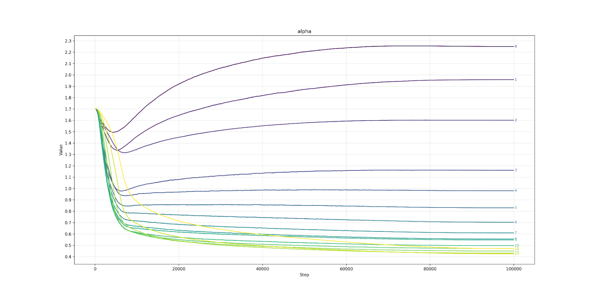
Alpha Llama3.2 1B
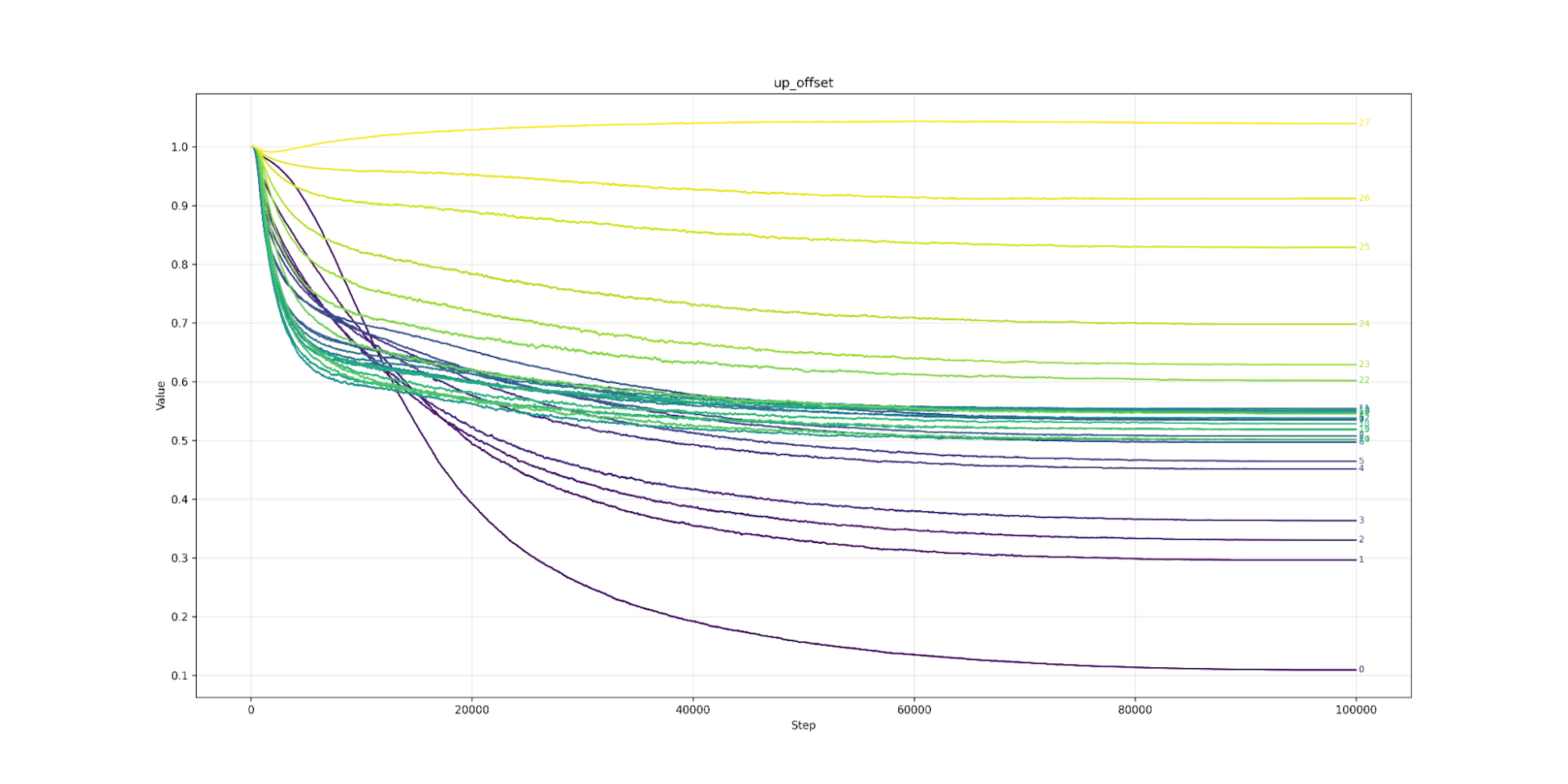
Up Offset Qwen3 0.6B
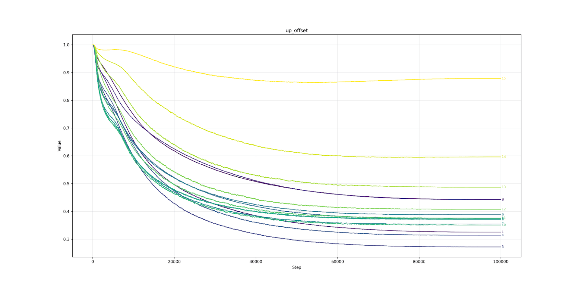
Up Offset Llama3.2 1B
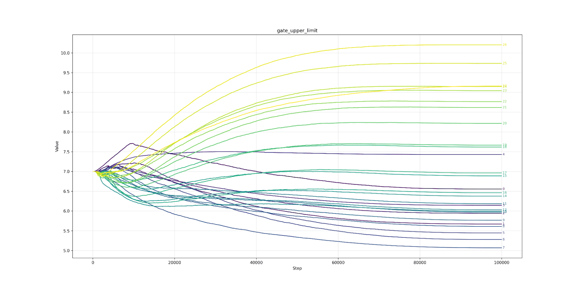
Gate Upper Limit Qwen3 0.6B

Gate Upper Limit Llama3.2 1B
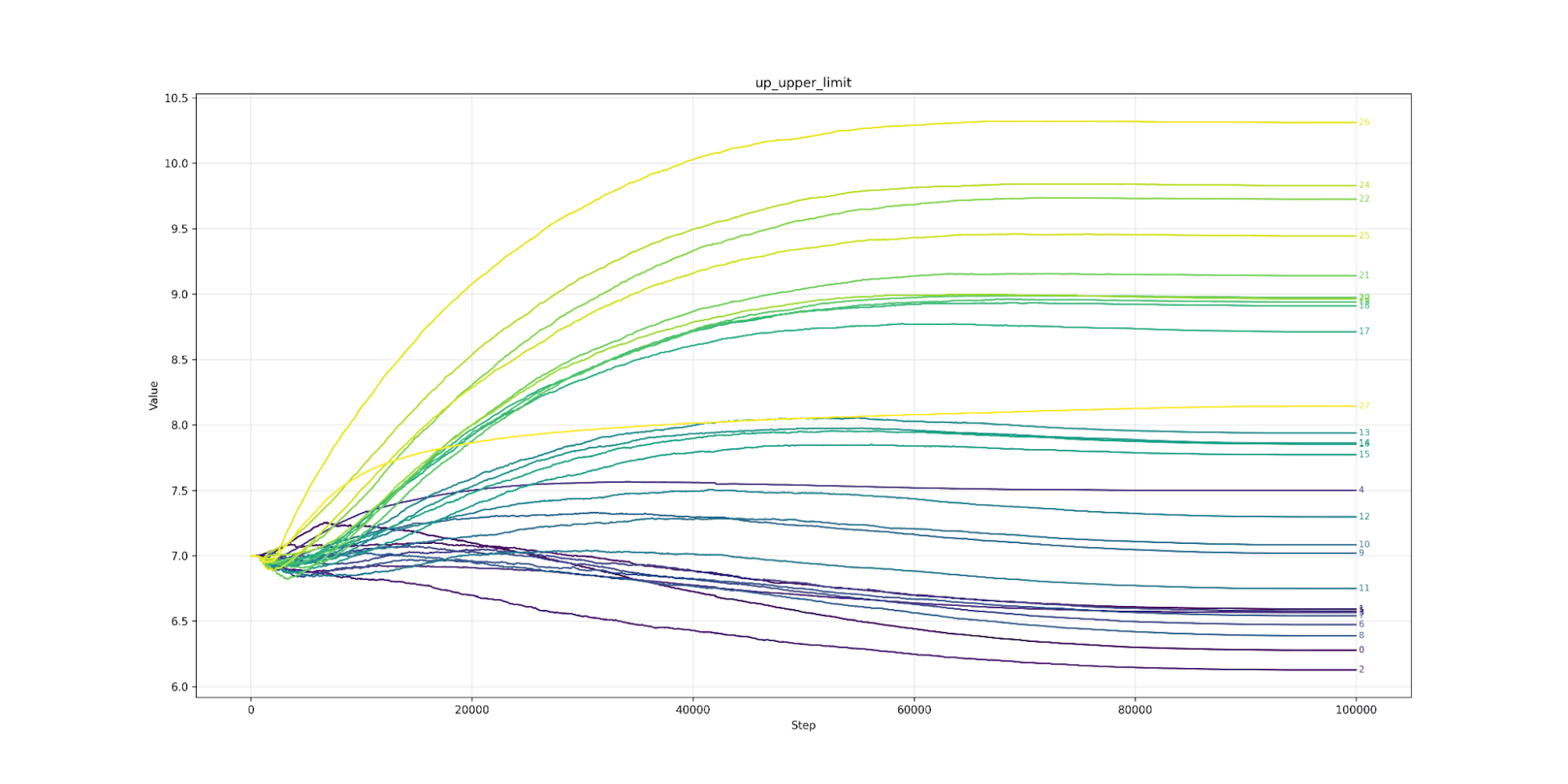
Up Upper Limit Qwen3 0.6B
Up Upper Limit Llama3.2 1B
Up Lower Limit Qwen3 0.6B
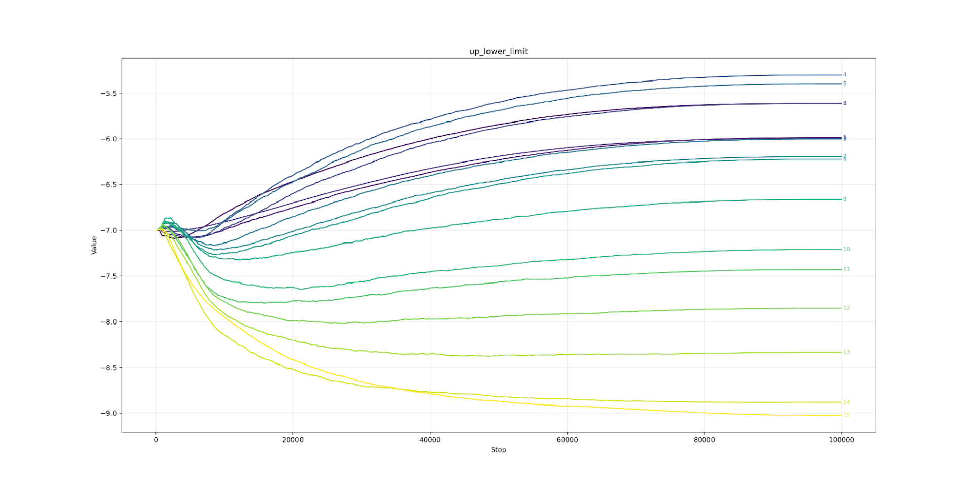
Up Lower Limit Llama3.2 1B